4  Mechanical Properties of Materials

NoteLearning Objectives

• Explain important mechanical properties of engineering materials, including representative behavior within an initial linear elastic region where stresses and strains are proportional to one another
• Describe how these material properties are determined, relating behavior on an actual specimen (a simple structure) to what the material experiences (local stresses and strains)
• Recognize different behavior of brittle and ductile materials and understand the important concept of yield strength
• Explore relationships among various moduli and Poisson’s ratio for linear elastic, isotropic materials
• Analyze linear elastic response of materials subjected to simple stress states, as well as the more complex multiaxial stresses imposed on real engineering products
• Apply a factor of safety as one simple means to begin to accommodate unexpected loading conditions, material variations, and other possible uncertainties

To meet design requirements of load-bearing structures typically involves determining the geometries and sizes of the components involved. For instance, a structure may have to be capable of carrying anticipated loads without failure (e.g., an aircraft wing), be stiff enough to deflect by only a limited amount (e.g., a building girder), or be material that returns to its original configuration when the loading is removed (e.g., a spring). To meet these design requirements we must understand the behavior of the material or materials being used within the structure. Exploring several of these basic mechanical properties is the focus of this chapter. An understanding of material behavior and these mechanical properties will enable us to relate stresses to strains, relate temperature change to strains, and explore the coupling that exists when subjecting materials to an arbitrary stress state.

The mechanical properties described in this chapter vary among materials. These properties can be measured and recorded for reference in engineering handbooks. Some useful properties for common engineering materials are recorded in Appendix C.

For the purposes of this book as we learn the principles, we assume that mechanical properties are constant—that is, independent of temperature, rate of loading, and other factors. This assumption works well for many engineering materials such as steel and aluminum at moderate temperatures, but not necessarily at very high temperatures. In addition, the mechanical properties of polymers, including plastics and rubber, are known for their temperature, time and rate dependence. That is, their properties change as these factors vary, often at common use temperatures. This makes presenting their properties in a simple table challenging. Practicing engineers often need to recognize and address such complications as they work with such materials.

Of particular importance is that materials in this text are assumed to be isotropic, which means they have the same properties in all directions. Many metals, polymers, concrete, and ceramics, including as discussed in this book, are often considered to be isotropic. Note that anisotropic materials, which display different properties depending on the direction of loading, are quite common but are beyond the scope of this text. Examples include wood, fiber-reinforced plastics such as fishing rods or airplane wing skins, and biological tissues such as tendon.

Section 4.1 discusses a common method of determining mechanical properties, known as the tensile test. The output of the tensile test—the stress-strain diagram—is analyzed in Section 4.2.

Important mechanical relationships, including Hooke’s law, which relates stress to strain, and Poisson’s ratio, which relates normal strain in the axial and lateral directions, are covered in Section 4.3 and Section 4.4 respectively.

Section 4.5 considers the relationship between shear stress and shear strain, and Section 4.6 introduces the concept of thermal strain. Section 4.7 expands Hooke’s law from Section 4.3 to the general three-dimensional case.

Finally, Section 4.8 focuses on applying a factor of safety to our designs to ensure they don’t fail.

4.1 Tensile Test

Click to expand

A common method of measuring mechanical properties of materials is the tensile test, which involves placing a cylinder or bar of material in a load frame (such as shown in Figure 4.1 (A)) and subjecting the specimen to tensile loading. A specimen (such as shown in Figure 4.1 (B)) is mounted in grips that are then separated at a prescribed displacement rate. Because of the likelihood of failures at the grip due to concentrations of stress, specimens are typically “waisted” to form dog bone or dumbbell shapes. Large fillets are used to reduce stress concentrations associated with the different areas (see Section 5.2), and failure typically occurs within the narrowed region of the specimen because of the smaller cross-sectional area. This region is often referred to as the gauge length, as this becomes the area of interest for the specimen.

The applied tensile load is steadily increased and along with the deformation of the specimen is measured and recorded at regular intervals. To determine deformation, a device such as a mechanical extensometer—see Figure 4.1 (C)—is mounted on the specimen. The specimen produces a uniform uniaxial stress state within its gauge region. For each data point, the load is used to calculate the average normal stress from Equation 2.1.

\[ \sigma=\frac{N}{A} \]

The deformation is used to calculate the average normal strain from Equation 3.1, where ΔL is the deformation measured by the strain gauge over the active length of the extensometer, L.

\[ \varepsilon=\frac{\Delta L}{L} \]

These quantities are essential in engineering design because properties from appropriate tests on laboratory specimens may be used to predict the behavior of much more complex engineering components.

Figure 4.1: Tensile tests are a common means to measure mechanic properties of materials. (A) Illustration of a tensile test frame. (B) Left to right: Examples of steel, aluminum, poly(vinyl chloride), and poly(methyl methacrylate) tensile specimens. (C) Image of a circular steel specimen mounted in grips and instrumented with a clip-on extensometer.

4.2 Stress-Strain Diagram

Click to expand

The goal in conducting tests of materials, such as the tensile test described above, is to learn qualitatively how the specimen responds to the applied loads and to quantitatively determine a material’s important mechanical properties.

As discussed in the introduction to this chapter, this text assumes these material properties to be constant and so, once determined from a test specimen, can be used to design and analyze components made of that same material. Appendix C contains material properties for a selection of these materials. Again, caution is needed as these properties can vary, sometimes substantially, depending on temperature, loading rate, prior loading history, and other factors.

The stress and strain data collected from a tensile test can be plotted to create a stress-strain diagram. Figure 4.2 illustrates an exaggerated stress-strain curve for a steel specimen. Let’s discuss the shape of the curve, the behavior of the material, and the material properties that can be determined from this plot.

4.2.1 Yield Stress

Initially a linear relationship exists between stress and strain, represented as a straight line on the stress-strain diagram. Following this is a plateau where a relatively small increase in stress results in a large increase in strain. The transition between the linear region of the stress-strain curve and the subsequent behavior marks an important engineering property of the material known as the yield stress, σ_yield.

There are actually three values worth mentioning here:

1. The point where the relationship between stress and strain stops being linear is known as the proportional limit, σ_PL.

2. Following the proportional limit is the elastic limit, σ_EL. If a material is loaded so that the stress does not exceed the elastic limit and then the load is removed, the object will return to its original dimensions. The elastic limit marks the point beyond which materials do not return to their original state.

3. The yield point is typically defined using the 0.2 percent offset method where a straight line beginning at a strain of 0.002 (0.2%) and running parallel to the linear portion of the diagram is drawn. The point where this line intersects the stress-strain curve is the yield point.

Since these three points for a material often occur within a fairly narrow range of one another, this text refers to these three points collectively as yielding. We use the yield stress because this is the easiest of the three points to consistently identify when working with real data.

Figure 4.2: Idealized stress-strain curve for a steel specimen, indicating the proportional limit (σ_PL), elastic limit (σ_EL), yield stress (σ_yield), ultimate tensile strength (σ_ultimate), and fracture stress (σ_fracture).

4.2.2 Elastic and Plastic Deformation

Prior to yielding, the material undergoes elastic deformation. If the load is removed during elastic deformation, the object will return to its original dimensions. This makes the yield strength of the material a highly important design parameter, as many engineering components are designed to operate within the linear region of material response and hence remain elastic.

When loaded past the yield point, the material continues to experience increasing stress and strain, though it is no longer a linear relationship. Deformation beyond the yield point is permanent. This is known as plastic deformation. If an object is loaded beyond its yield point and the load is then removed, any elastic deformation is recovered but any plastic deformation is not. The object’s dimensions have been permanently changed.

You likely have experienced material yielding if you have ever deformed a coat hanger or paperclip such that it doesn’t return to the original state. Such behavior is undesirable for many engineering components designed to continue operating in their original state, so engineers commonly consider the yield stress to be the maximum acceptable stress in a component.

However, plastic deformation following yielding can be very important in the fabrication process. For example, sheets of steel or aluminum can be placed between molds and compressed under high pressure to deform them into the shape of an automobile panel as seen in Figure 4.3 (A). Plastic deformation can also be useful in absorbing energy, such as seen in the concertina crushing of a structural component for an automobile, shown in Figure 4.3 (B). This book, however, focuses on the pre-yield, linear elastic region.

Figure 4.3: Engineering materials are often loaded beyond yield to permanently deform the material, as in (A) the stamping process for an automotive panel or in (B) the crushing of a weld-bonded hat section used to absorb energy in an automobile accident.

If we continue to load the specimen into the plastic region, the stress and strain continue to increase until some maximum stress known as the ultimate tensile stress, σ_UTS. Past this point the material undergoes necking—a thinning of the cross-section—and so the load it can withstand actually decreases. This continues until the fracture point, σ_fracture.

4.2.3 Ductile and Brittle Materials

Figure 4.2 shows an idealized stress-strain diagram for a steel specimen. The diagrams for other materials will look a little different because their mechanical properties are all different. Figure 4.4 (A) illustrates representative stress-strain behavior for several engineering materials. These are drawn to scale, and the popout shows an enlarged view of the elastic region.

Each material initially experiences a linear relationship between stress and strain, but the yield stress is significantly higher for some materials than others. Materials with a high yield stress are of course more appropriate for high-stress applications.

Figure 4.4: Results obtained from tensile tests. (A, left) Illustration of typical stress-strain behavior for some common materials. Temperatures denote anneal temperatures. (A, right) Same data plotted up to 5 percent strain. (B) Tensile test of an AlMgSi alloy. This is a ductile fracture type, as seen by the local necking and the cup and cone fracture surfaces.

Consider the plastic deformation for the materials shown in Figure 4.4. Some materials, such as cast iron, fail at relatively small strains, whereas other materials, such as high-density polyethylene (HDPE) often used for milk jugs, reach very large strains well beyond the axis limit.

Brittle materials are those with short plastic regions, indicating they break without experiencing much plastic deformation. The behavior remains nearly linear until failure.

Ductile materials are those with long plastic regions, indicating they experience significant plastic deformation before breaking. Figure 4.4 (B) shows the failure region of an aluminum alloy specimen tested to failure, illustrating necking and ductile failure. This can be useful in many engineering applications where the material will deform significantly if the yield stress is accidentally exceeded and can thereby allow time for the component to be replaced before it breaks. Consider the difference between dropping a ceramic mug on a hard floor compared to a mug made of aluminum or tin. The ceramic mug is likely to shatter, whereas the tin mug may end up with a permanent dent (indicating that its yield stress was exceeded and it experienced plastic deformation) but will still be functional.

4.3 Hooke’s Law

Click to expand

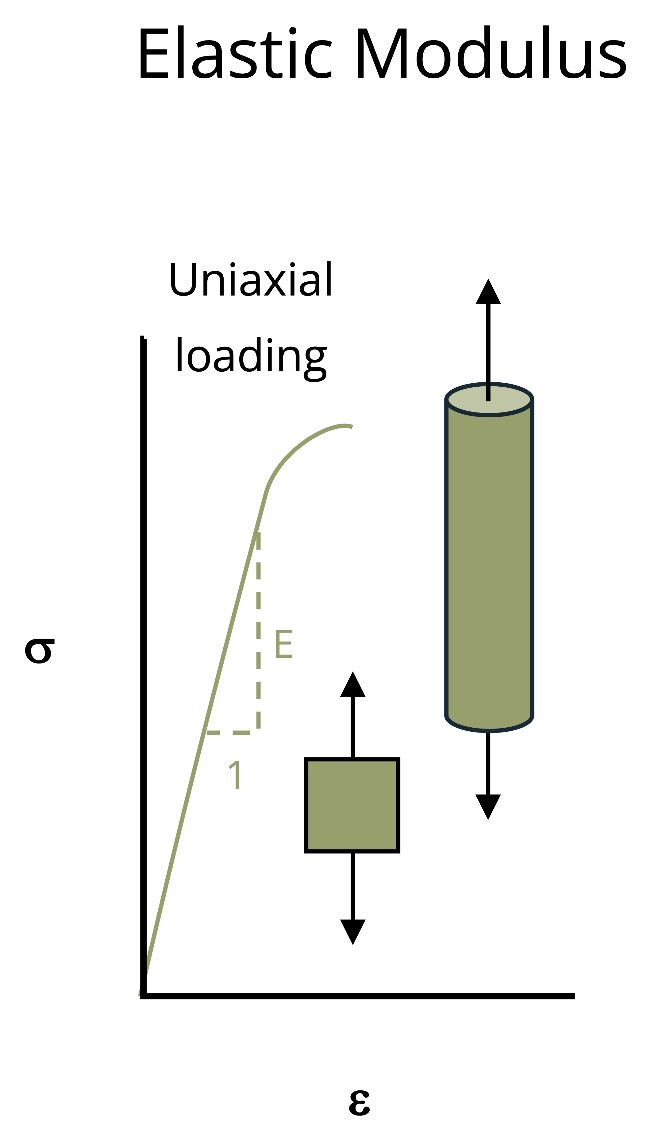
The slope of the linear region of this stress-strain diagram represents an important material property known as the elastic modulus (also known as Young’s modulus or the modulus of elasticity), so designated by E. Thomas Young (1773-1829), a British scientist who noted the proportionality between applied force and extension, which he recorded as ut tensio sic vis, meaning “as is the extension, so is the force.”

The elastic modulus can be thought of as a measure of stiffness of the material. A high elastic modulus for stiff materials is represented by a steep slope—that is, a large increase in stress with only a small increase in strain. A low elastic modulus for soft materials is represented by a shallow slope, indicating a small increase in stress but a large increase in strain.

The linear elastic region of material response is of enormous importance for most engineering structures. Loading significantly beyond this proportional limit can result in pronounced yielding and permanent deformation that is often unacceptable, unless one is using this deformation to absorb energy (as in an automobile frame involved in collision). The elastic modulus is illustrated in Figure 4.5, which plots a portion of the normal stress versus normal strain, for example, from a tensile test.

\[ E=\frac{\sigma}{\varepsilon} \]

Since strain is unitless, elastic modulus will have the same units as stress (Pa or psi).

This relationship is more commonly called Hooke’s law, and written as

\[ \boxed{\sigma=E \varepsilon}\text{ ,} \tag{4.1}\]

where
𝜎 = Average normal stress [Pa, psi]
E = Elastic modulus [Pa, psi]
𝜀 = Normal strain

This equation is appropriate for uniaxial stress (i.e., when the load is applied and the strain measured in only the same single direction). Section 4.7 expands this relationship to cases where normal stresses occur in more than one direction.

Especially important to note is that this relationship is applicable only within the linear elastic region of the material’s response. This relationship, applicable at the material level for stress and strain, also extends to structural elements (e.g., bars in tension or compression, beam deflections, or helical springs in which the force and deflection are related by the spring constant) and many other engineering components and structures, as covered in the following chapters of the book.

Figure 4.5: Illustration of the initial linear elastic portions of the stress-strain curve and slope corresponding to elastic modulus for uniaxial tension.

Example 4.1 uses Hooke’s law to determine the elastic modulus of a material where the applied load and deformation are known.

TipExample 4.1

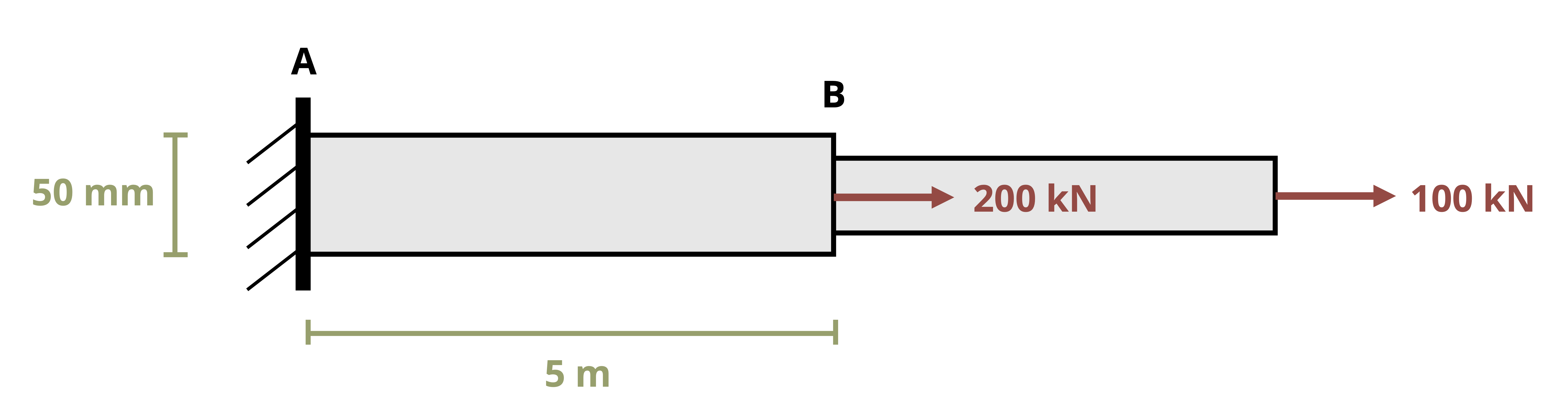
Example 4.1  

Two bars are welded together and fixed to a wall at A. Two loads are applied as shown. Bar AB is 5 m long and has a diameter of 50 mm.

If the change in length of bar AB is 4 mm, determine the elastic modulus of this bar.

TipSolution

Cut a cross-section through bar AB and determine the internal load.

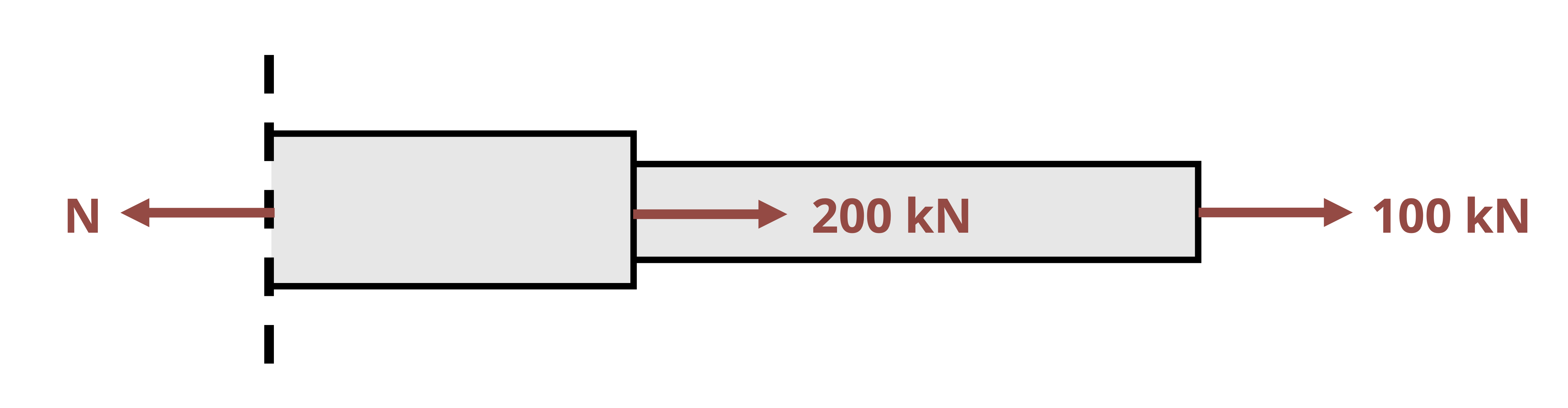
\[ \sum F_x= 100{~kN}+200{~kN}-N=0 \quad\rightarrow\quad N=300{~kN} \]

Calculate the normal stress.

\[ \sigma=\frac{N}{A}=\frac{300,000{~kN}}{\pi(0.025)^2{~m}^2}=152.8{~MPa} \]

Calculate the normal strain.

\[ \varepsilon=\frac{\Delta L}{L}=\frac{4{~mm}}{5,000{~mm}}=0.0008 \]

Use Hooke’s law to calculate the elastic modulus. \[ E=\frac{\sigma}{\varepsilon}=\frac{152.8 \times 10^6{~Pa}}{0.0008}=191{~GPa} \]

WarningStep-by-Step: Elastic Modulus

1. Determine the internal load in the member by equilibrium.
2. Determine the normal stress in the member by \(\sigma=\frac{N}{A}\).
3. Determine the normal strain in the member by \(\varepsilon=\frac{\Delta L}{L}\).
4. Use Hooke’s law to calculate the elastic modulus, \(\sigma=E \varepsilon\).

4.4 Poisson’s Ratio

Click to expand

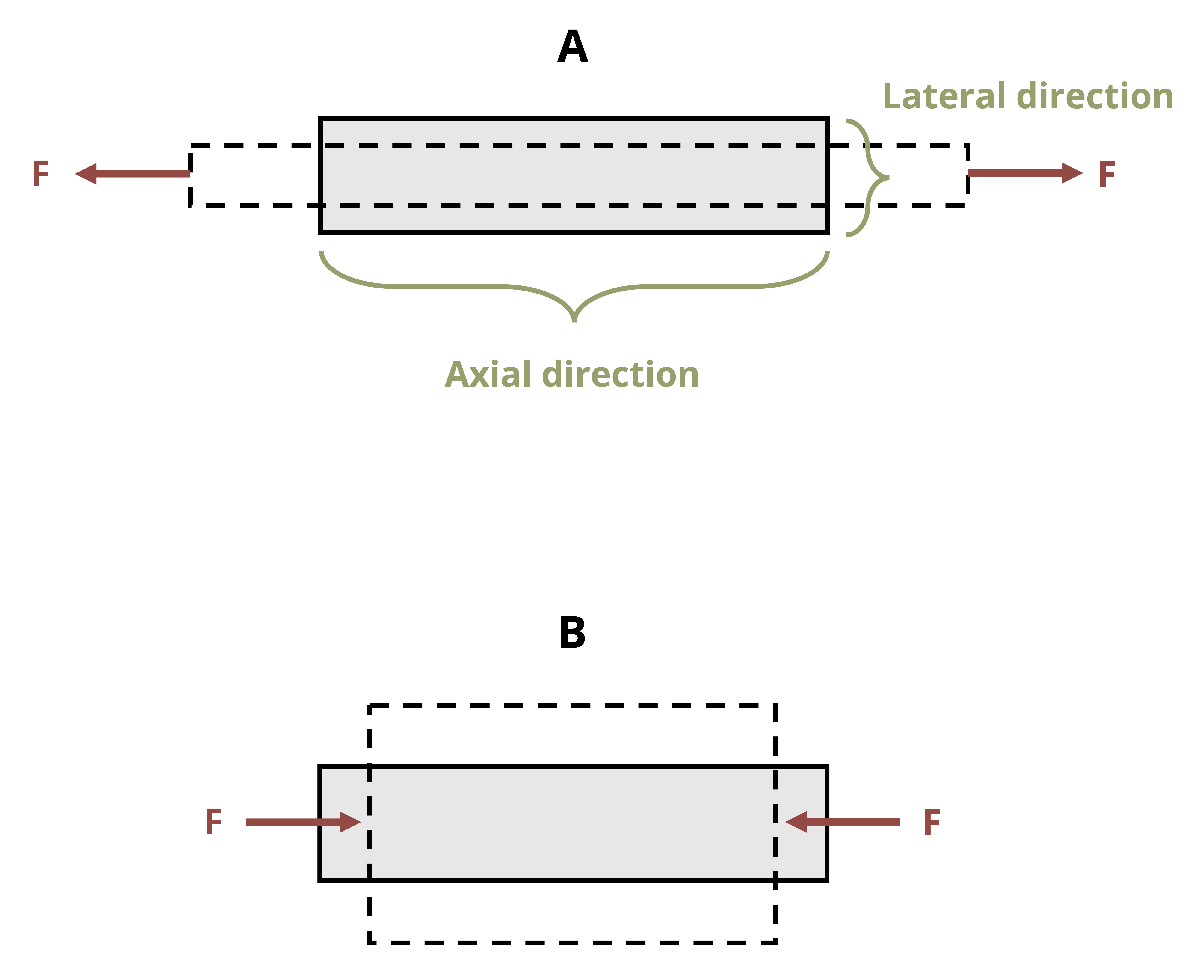
When you stretch a rubber band, you’ll notice that the band gets longer in the direction of the applied force, but the width of the band decreases. That is, a normal strain occurs in the axial (length) direction and also in the lateral (width or thickness) direction. These normal strains couple in perpendicular directions. Poisson’s ratio is the material property that describes the proportional relationship between axial and lateral strains. Named after Siméon Denis Poisson (1781-1840), the French mathematician and physicist, Poisson’s ratio is defined as the negative of the lateral strain divided by the axial strain for a uniaxially loaded material. It may be expressed as

\[ \boxed{\nu=-\frac{\varepsilon_{lateral}}{\varepsilon_{axial}}}\text{ ,} \tag{4.2}\]

where
𝜈 = Poisson’s ratio
𝜀_lateral = Lateral normal strain
𝜀_axial = Axial normal strain

Recall that strains are positive if the dimension lengthens and negative if it shortens. For most common engineering materials, applying a tensile force causes the object to become longer and thinner, while applying a compressive force causes it to become shorter and wider. This is shown in Figure 4.6. Thus, for these materials, either the axial or lateral strain will be positive and the other will be negative.

Figure 4.6: Illustration of axial and lateral strains for (A) Tensile loading and (B) Compressive loading. Solid lines show original (undeformed) shape, and dotted lines show deformed shape. Note that one strain is positive (elongating) and the other is negative (shortening) in both cases.

Note that this relationship is appropriate for a uniaxially loaded specimen. Section 4.7 expands this relationship to cases of normal stresses in more than one direction.

Poisson’s ratio depends on the material as well as its structure. Theoretically, Poisson’s ratio can range from –1 to +0.5 for isotropic materials but usually ranges from near zero for foams to almost exactly 0.5 for soft materials such as elastomers and gels. Most metals fall in the range from 0.2 to 0.35. A positive value of Poisson’s ratio means that as the material is extended in one direction, a contraction occurs in lateral directions. See Example 4.2 for a simple application of Poisson’s ratio.

TipExample 4.2

Example 4.2  

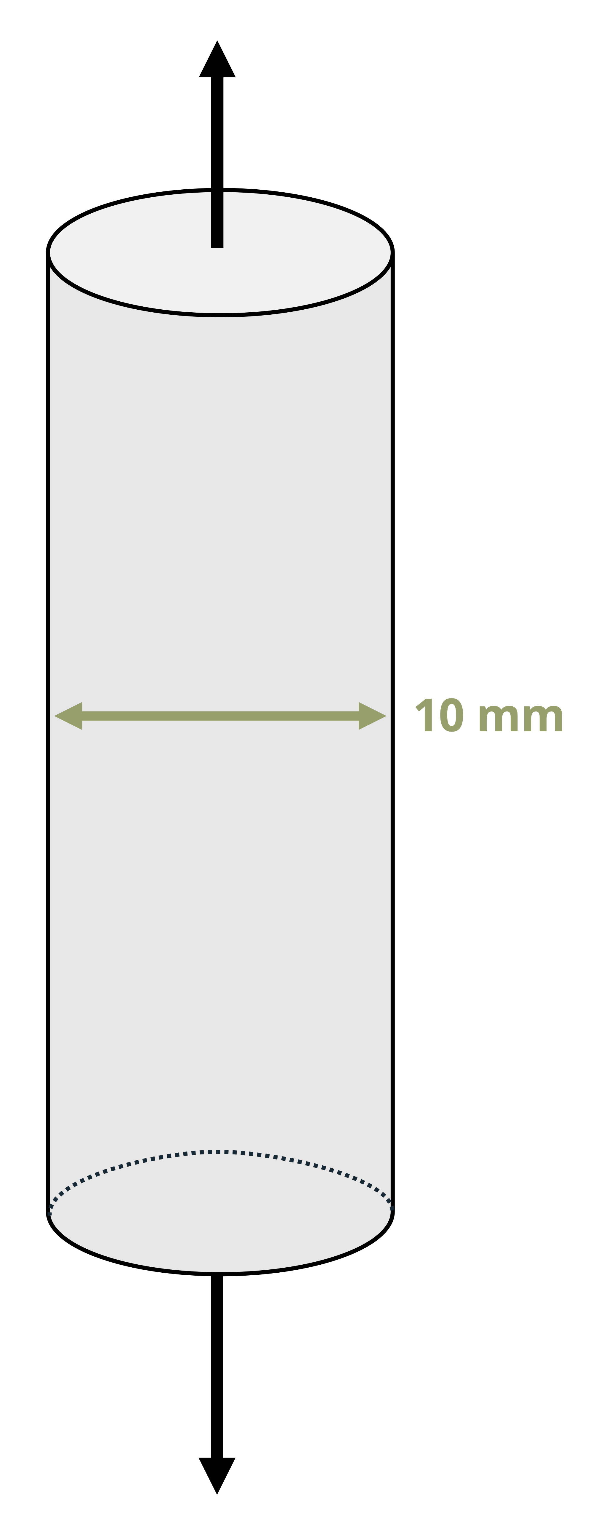
A circular polymeric rod with a diameter of 10 mm is subjected to a uniaxial force, resulting in an axial strain of 0.5%. A corresponding reduction in diameter of 0.02 mm is measured.

Determine the Poisson’s ratio of this material.

TipSolution

The longitudinal strain is given as ε_longitudinal = 0.005.

The lateral strain is determined from the reduction in diameter divided by the original diameter and is negative because it is contracting.

\[ \varepsilon_{lateral}=-\frac{0.02~mm}{10~mm}=-0.002 \]

Poisson’s ratio is then easily determined as

\[\nu=-\frac{\varepsilon_{lateral}}{\varepsilon_{axial}}=-\frac{-0.002}{0.005}=0.4\]

WarningStep-by-Step: Poisson’s Ratio

1. Determine the axial strain, given the change in length (L): \(\varepsilon_{axial}=\frac{\Delta L}{L}\).

2. Determine the lateral strain, given the change in diameter (D), height (H), or width (W): \(\varepsilon_{l a t}=\frac{\Delta D}{D}=\frac{\Delta H}{H}=\frac{\Delta W}{W}\).

3. Calculate Poisson’s ratio: \(\nu=-\frac{\varepsilon_{lateral}}{\varepsilon_{axial}}\).

4.5 Shear Stress and Strain

Click to expand

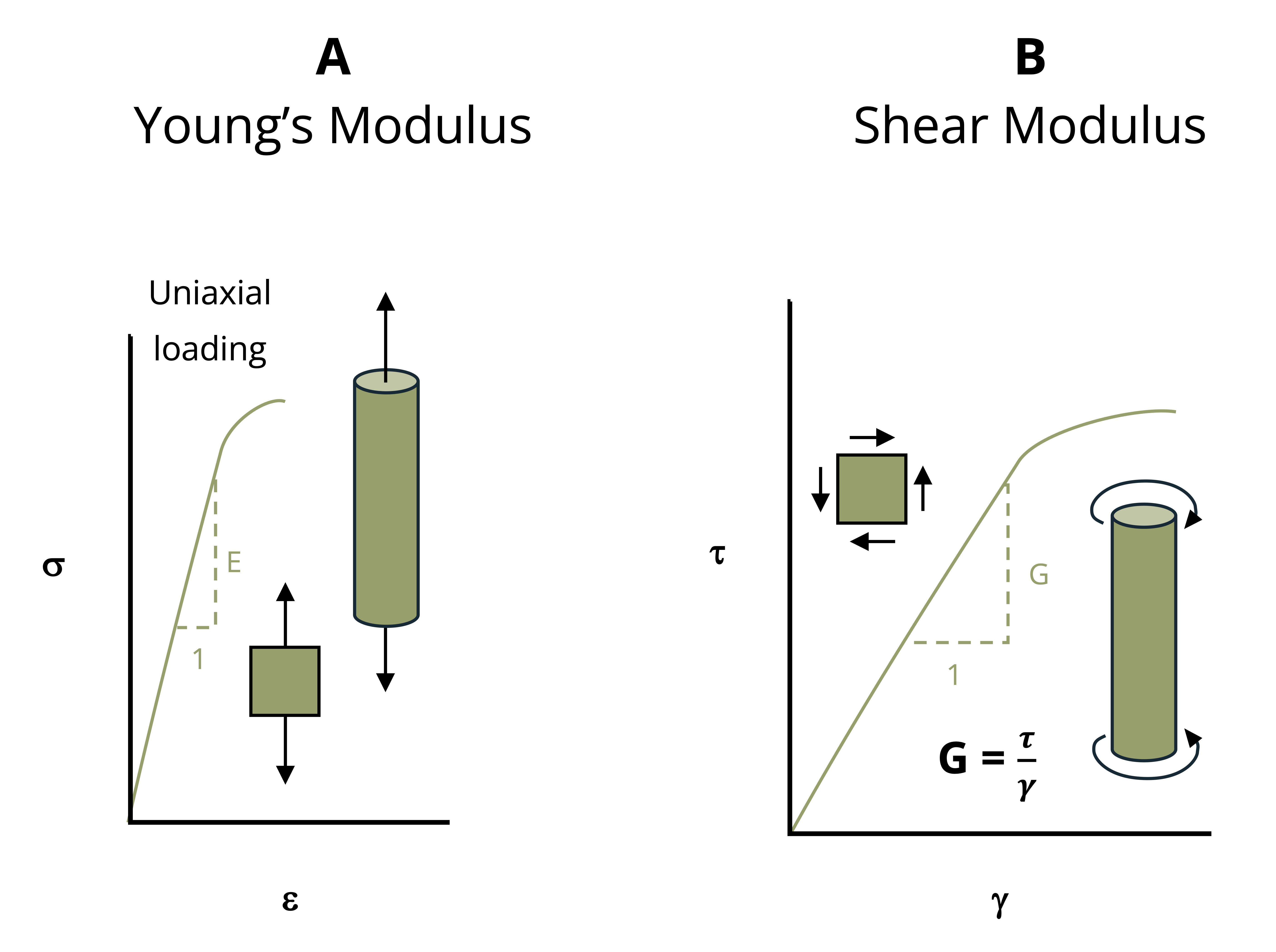
In addition to considering normal stresses and strains, engineers require an understanding of the relationship between shear stresses and shear strains. Like the tensile test for normal stress and strain, a shear test can be performed to produce a diagram of shear stress against shear strain. The slope of a shear stress versus shear strain diagram is referred to as the shear modulus or modulus of rigidity and is designated by G. The corresponding slope of a shear stress versus shear strain plot is referred to as the shear modulus or modulus of rigidity, as shown in Figure 4.7 (B).

\[ \boxed{\tau=G \gamma}\text{ ,} \tag{4.3}\]

where
𝜏 = Shear stress [Pa, psi]
G = Shear modulus or modulus of rigidity [Pa, psi]
𝛾 = Shear strain

Figure 4.7: Illustration of the initial linear elastic portions of the stress-strain curve and slopes corresponding to (a) Young’s modulus for uniaxial tension; (b) shear modulus for pure shear loading

Noted that the elastic modulus, the shear modulus, and Poisson’s ratio are not independent of each other. For isotropic materials, only two are independent, linear elastic properties; knowing any two allows us to calculate the others. It can be shown that

\[ \boxed{G=\frac{E}{2(1+v)}}\text{ ,} \tag{4.4}\]

where
G = Shear modulus or modulus of rigidity [Pa, psi]
E = Elastic modulus [Pa, psi]
𝜈 = Poisson’s ratio

See Example 4.3 for a problem involving the shear modulus.

TipExample 4.3

Example 4.3  

Soft contact lenses often consist of a hydrogel, an elastomeric network that is imbibed with water, expanding its volume and making the lens more soft and compliant.

Suppose a 10 mm cube of the dry elastomer were subjected to a shearing action as shown. Shearing forces of 5 N each are applied to the four faces of the cube, resulting in a displacement of 0.3 mm.

What is the shear modulus of this elastomeric block?

TipSolution

First determine the shear stress.

\[ \begin{aligned} &A=L^2=(0.01~m)^2 \\ &\tau=\frac{V}{A} \\ & \tau=\frac{5{~N}}{(0.01{~m})^2}=50{~kPa} \\ \end{aligned} \]

Then determine the shear strain.

\[ \begin{aligned} & \gamma = \frac{\Delta x}{L}\\ & \gamma=\frac{0.3{~mm}}{10{~mm}}=0.03 \\ \end{aligned} \]

Finally, calculate the shear modulus.

\[ G=\frac{\tau}{\gamma}=50{~kPa}/0.03=1.667{~MPa} \]

WarningStep-by-Step: Shear Modulus

1. Determine the internal load in the member by equilibrium.
2. Determine the shear stress in the member by \(\tau=\frac{V}{A}\).
3. Determine the shear strain in the member by \(\gamma=\frac{\Delta x}{L}\).
4. Use Hooke’s law to calculate the shear modulus, \(\tau=G \gamma\).

4.6 Thermal Strain

Click to expand

Other factors in addition to relationships arising between load, stress, and strain, can affect dimensional changes of materials as well as changes in the stresses present in a structure. Most materials will expand, for example, when their temperature is increased. Many engineering structures will experience significant temperature variations during their life, beginning with thermal processes involved in their manufacture, cyclic temperature changes (e.g., day/night or summer/winter), or because of their usage, such as an engine block heating up or cooling down. Although dimensional changes from temperature often appear to be quite small, they can lead to significant changes in stress state, and in fact numerous failures result not from applied mechanical loading but from thermal exposure issues. Though beyond the current scope, dimensional changes can also result from other environmental factors, such as the expansion of a material as water is absorbed, or from the application of electric fields for materials that exhibit piezoelectric properties.

Vibrational energy of atoms increases as temperature increases, typically leading to slightly greater atomic separation distances. This expansion leads to dimensional changes in the material, and the behavior is characterized by the material’s coefficient of thermal expansion (CTE). The linear CTE is often designated by \(\alpha\) and is defined as the change in strain per unit change in temperature. As with the other material properties discussed in this chapter, ⍺ is assumed to be constant for any given material.

The CTE is independent of direction in isotropic materials. We can determine the CTE by heating or cooling a specimen and measuring the resulting strain (ε) or dimensional change and recording the change in temperature (ΔT).

\[ \alpha=\frac{\varepsilon}{\Delta T}=\frac{\frac{\Delta L}{L}}{\Delta T}\text{,} \]

where \(\Delta T=T_{final}-T_{initial}\). Since strain is unitless, CTE has units of \(\frac{1}{{ }^{\circ} \mathrm{C}}\) or \(\frac{1}{{ }^{\circ} F}\). Knowing the CTE enables us to easily determine the strain expected when a material is subjected to a temperature change of ΔT.

\[ \boxed{\varepsilon_T=\alpha \cdot \Delta T} \tag{4.5}\]

Or dimensional changes can be determined as

\[ \boxed{\Delta L=\alpha \cdot \Delta T \cdot L}\text{ ,} \tag{4.6}\]

where
𝜀_T = Thermal strain
𝛼 = Coefficient of thermal expansion \(\left[\frac{1}{^\circ C},\frac{1}{^\circ F}\right]\)
𝛥T = Change in temperature \([^\circ C, ^\circ F]\)
𝛥L = Change in length [m, in.]
L = Original length [m, in.]

See Example 4.4 for a problem involving a temperature change resulting in a thermal strain.

TipExample 4.4

Example 4.4  

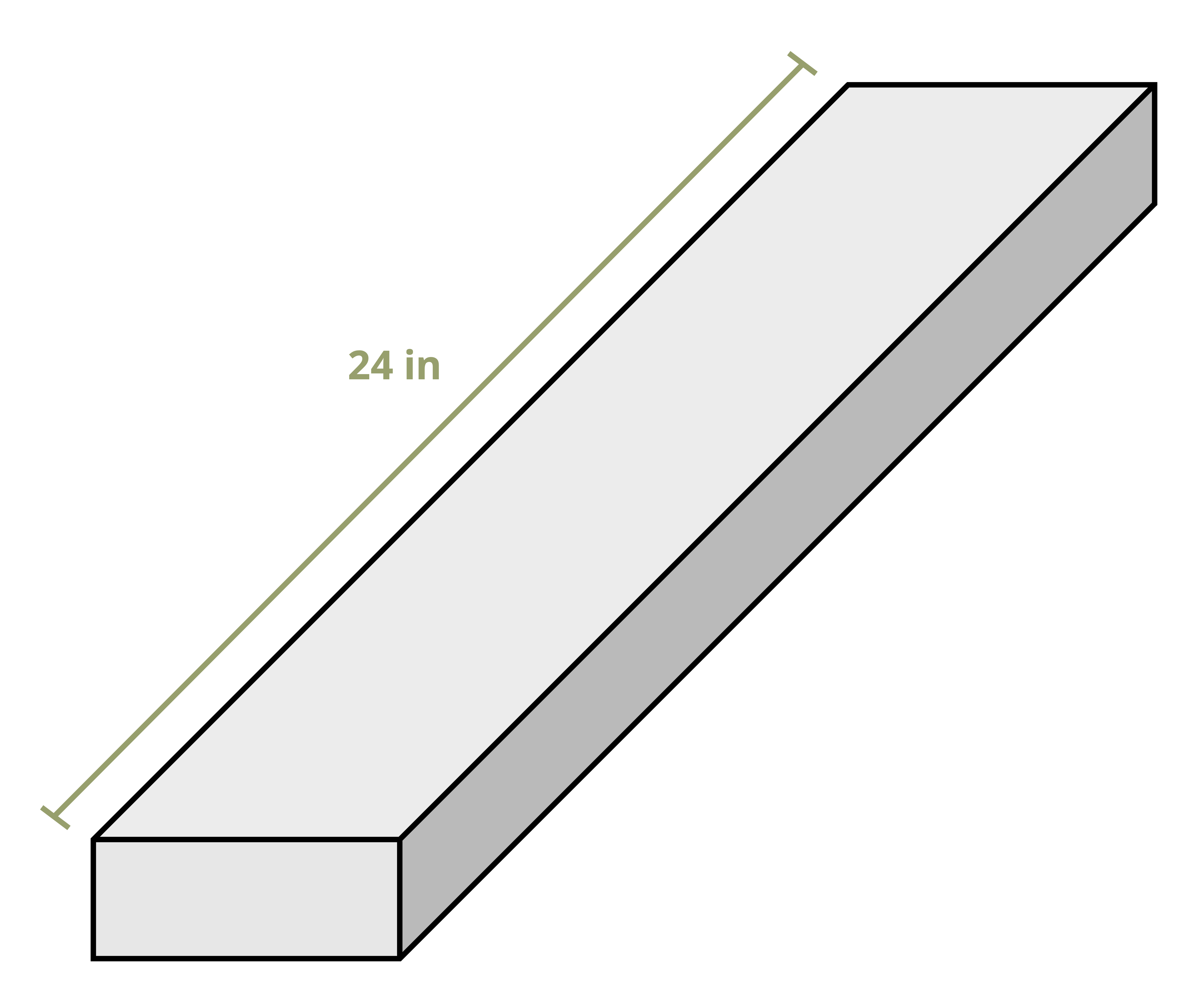
A 24 in. long aluminum bar with a coefficient of thermal expansion of 13 x 10^-6/F° and Young’s modulus of 10,000 ksi is cooled from 100 °F to 25 °F.

1. What change in strain results from this temperature change if the bar is free to contract?
2. What change in length results from this temperature change if the bar is free to contract?

TipSolution

1. Thermal strain can be calculated from \(\varepsilon_T=\alpha \Delta T\).

   \(\varepsilon_T=\alpha \cdot \Delta T\\ \varepsilon_T=13 \times 10^{-6} /^\circ{F} *\left(-75^{\circ}{F}\right)\\ \varepsilon_T=-0.00098\)

2. Change in length can be determined from \(\varepsilon=\frac{\Delta L}{L}\).

   \(\varepsilon = \frac{\Delta L}{L} \quad \rightarrow\quad\Delta L=\varepsilon L\\ \Delta L=-0.00098*24{~in.}\\ \Delta L=-0.0235 {~in.}\)

WarningStep-by-Step: Thermal Strain

1. Determine the change in temperature, \(\Delta T=T_{final}-T_{initial}\).

2. Look up the coefficient of thermal expansion (𝛼) for the material.

3. Calculate the thermal strain, \(\varepsilon_T=\alpha \Delta T\).

4. Calculate the change in length from \(\varepsilon=\frac{\Delta L}{L} \rightarrow \Delta L=\varepsilon L\).

4.7 Multiaxial or Generalized Hooke’s Law

Click to expand

Materials are often tested under idealized conditions (e.g., uniaxial tension or shearing resulting from torsional loading). These tests are important because they provide material properties necessary for engineering design. Such simple stress states are less common in actual engineered components, where more complex, multiaxial stress states are present, as shown in Figure 4.8.

Figure 4.8: Illustration of a general, multiaxial stress state, showing normal and shear stresses acting on the positive x-, y-, and z-planes. Note that equal and opposite stresses exist on the hidden faces of the element.

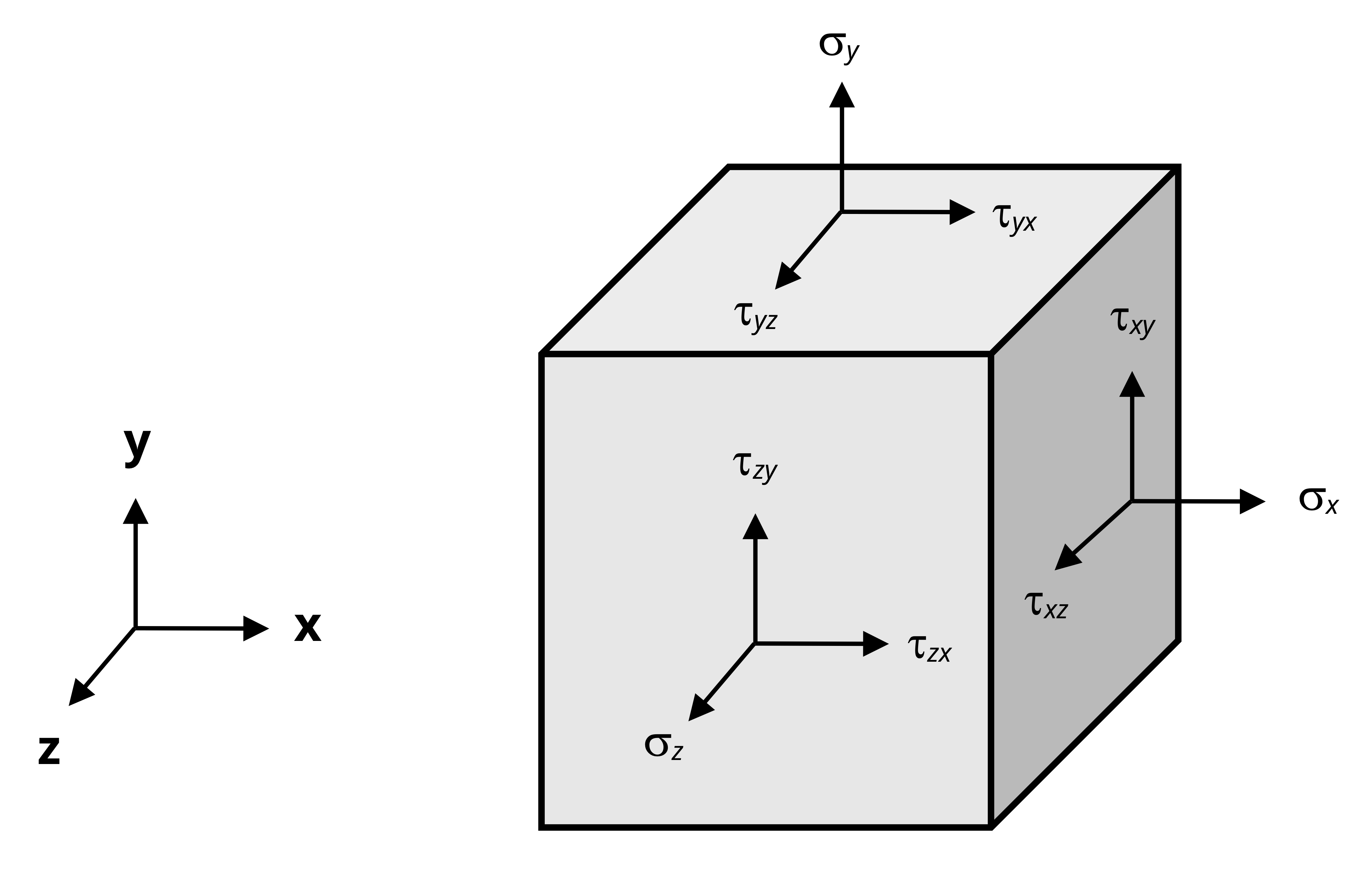
Here there are three normal stresses, referred to with a single subscript indicating their direction (σ_x, σ_y, and σ_z), though some texts use repeated subscripts for these (σ_xx, σ_yy, and σ_zz). There are six shear stresses, designated by τ. These are referred to with two subscripts, one indicating the plane or “face” the stress acts on and the other indicating the direction it acts in. For example, on the y-z plane (the x-face) are the normal stress σ_x and two shear stresses, τ_xy and τ_xz. The first subscript indicates that these shear stresses act on the x-face, and the second subscript indicates that they point in the y and z directions respectively.

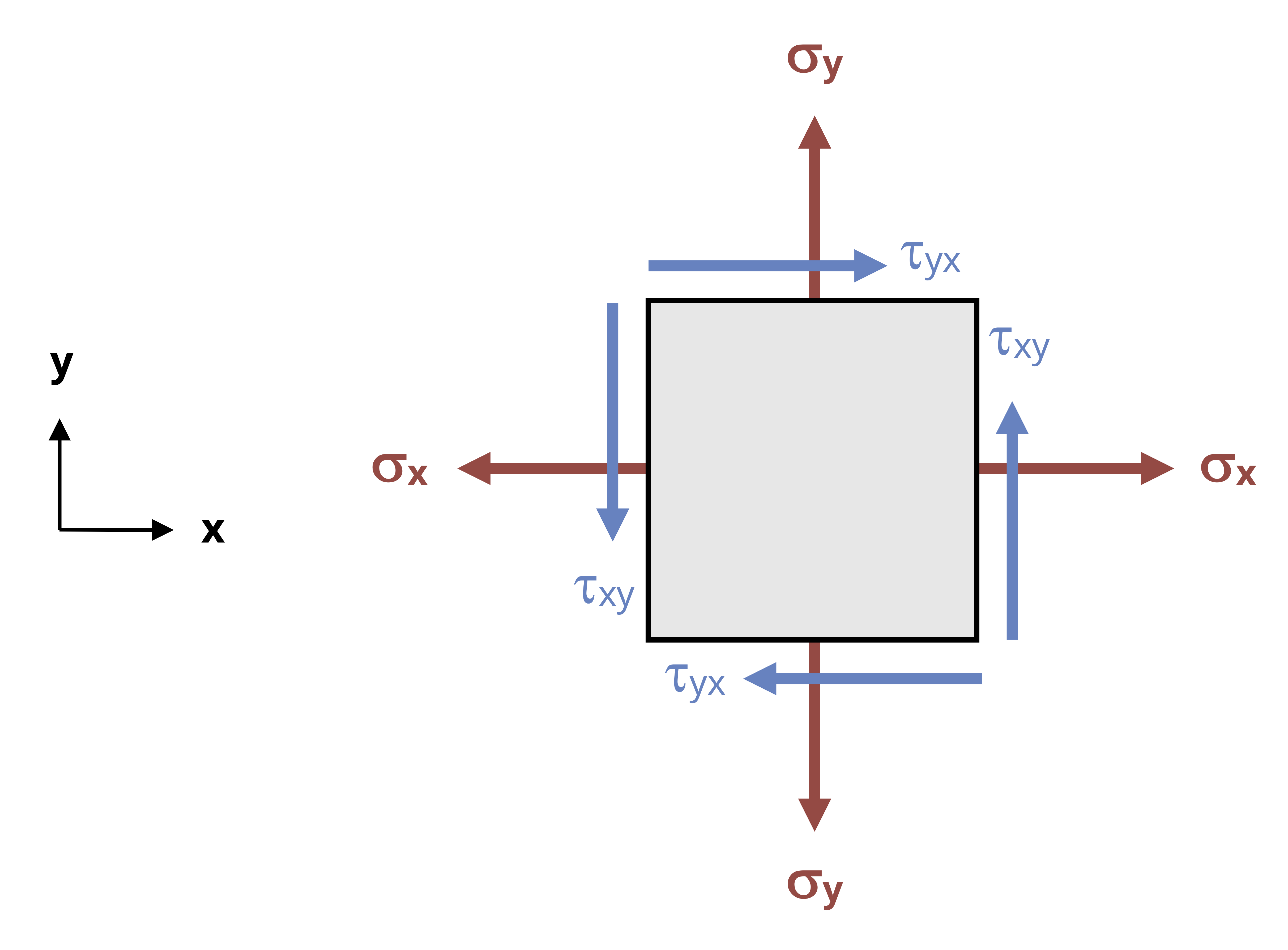
Consider the x-y plane of the stress element in Figure 4.8. This two-dimensional plane is shown in Figure 4.9. It experiences two normal stresses (σ_x and σ_y) and two shear stresses (τ_xy and τ_yx). Of these, τ_xy will cause the element to rotate counterclockwise, whereas τ_yx will cause the element to rotate clockwise. For an element in equilibrium, these two stresses must be equal for these rotation effects to balance. Expanding this to the other planes, τ_xy = τ_yx, τ_xz = τ_zx, and τ_yz = τ_zy.

Figure 4.9: 2D view of the x-y plane of a 3D stress element.

Given the concept of Poisson’s ratio, recognize that a normal stress in one direction creates normal strains in all three directions (x, y, and z). We have reviewed this in responding to the application of a uniaxial stress state—a normal stress applied in only one direction. For example, a normal stress in the x direction means there will be a normal strain in the x direction and also in the y and z directions.

\[ \begin{aligned} & \varepsilon_x=\frac{\sigma_x}{E} \\ & \varepsilon_y=-v \varepsilon_x=-\frac{\nu \sigma_x}{E} \\ & \varepsilon_z=-\nu \varepsilon_x=-\frac{\nu \sigma_x}{E} \end{aligned} \]

Most engineering structures, however, involve more complex stress states, in which stresses may be applied in the x, y, and z directions. We refer to these as multiaxial stress states. We can define similar equations for a normal stress applied in the y direction.

\[ \begin{aligned} & \varepsilon_y=\frac{\sigma_y}{E} \\ & \varepsilon_x=-\nu \varepsilon_y=-\frac{\nu \sigma_y}{E} \\ & \varepsilon_z=-\nu \varepsilon_y=-\frac{\nu \sigma_y}{E} \end{aligned} \]

And we can do likewise for a normal stress applied in the z direction.

\[ \begin{aligned} & \varepsilon_z=\frac{\sigma_z}{E} \\ & \varepsilon_x=-\nu \varepsilon_z=-\frac{\nu \sigma_z}{E} \\ & \varepsilon_y=-\nu \varepsilon_z=-\frac{\nu \sigma_z}{E} \end{aligned} \]

If loads are applied in all three directions simultaneously, we can determine the overall strain in each direction by simply adding together the above components.

\[ \boxed{\begin{aligned} & \varepsilon_x=\frac{\sigma_x}{E}-\frac{\nu \sigma_y}{E}-\frac{\nu \sigma_z}{E}=\frac{1}{E}\left[\sigma_x-\nu\left(\sigma_y+\sigma_z\right)\right] \\ & \varepsilon_y=\frac{1}{E}\left[\sigma_y-\nu\left(\sigma_x+\sigma_z\right)\right] \\ & \varepsilon_z=\frac{1}{E}\left[\sigma_z-\nu\left(\sigma_x+\sigma_y\right)\right] \end{aligned}}\text{ ,} \tag{4.7}\]

where
𝜀_x, 𝜀_y, 𝜀_z = Normal strain in the x, y, and z directions
𝜎_x, 𝜎_y, 𝜎_z = Normal stress in the x, y, and z directions [Pa, psi]
E = Elastic modulus [Pa, psi]
𝜈 = Poisson’s ratio

This is the generalized Hooke’s law for the three-dimensional state of stress. Example 4.5 demonstrates the application of the generalized Hooke’s law to a problem with stresses acting in the x, y, and z directions.

Similarly, normal strains are written with a single subscript as ε_x, ε_y, and ε_z, whereas shear strains are written with two subscripts as 𝛾_xy = 𝛾_yx, 𝛾_xz = 𝛾_zx, and 𝛾_yz = 𝛾_zy.

The relationships between shear stresses and strains do not change in isotropic materials subjected to additional other stress components, so

\[ \boxed{\begin{aligned} & \gamma_{xy}=\frac{\tau_{xy}}{G} \\ & \gamma_{yz}=\frac{\tau_{yz}}{G} \\ & \gamma_{xz}=\frac{\tau_{xz}}{G} \end{aligned}}\text{ ,} \tag{4.8}\]

where
𝛾_xy, 𝛾_yz, 𝛾_xz = Shear strains
𝜏_xy, 𝜏_yz, 𝜏_xz = Shear stresses [Pa, psi]
G = Shear modulus [Pa, psi]

TipExample 4.5

Example 4.5  

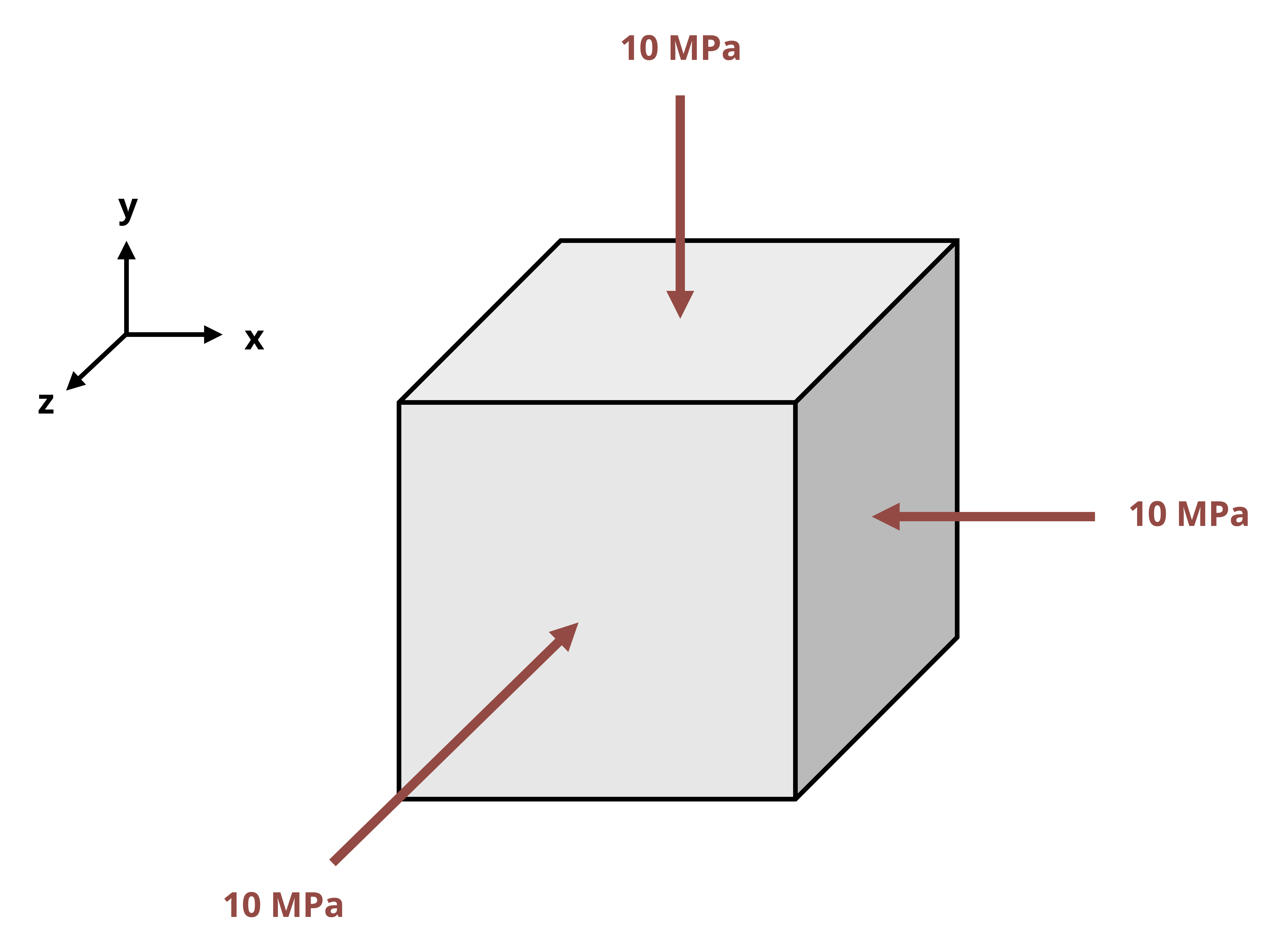
A solid, 50 mm polycarbonate cube is subjected to a compressive stress of σ = 10 MPa on all sides.

Assuming the material has a Young’s modulus of 3 GPa and a Poisson’s ratio of 0.38, what is the change in length of one of the edges?

TipSolution

First, note that a compressive stress acts in all directions, so σ_x = σ_y = σ_z = -10 MPa. We can choose any one of the generalized Hooke’s law equations to determine the strain in the corresponding direction, but note that all normal strains will be the same.

\[ \begin{aligned} & \varepsilon_x=\frac{1}{E}\left[\sigma_x-v\left(\sigma_y+\sigma_z\right)\right] \\ & \varepsilon=\frac{-\sigma}{E}[1-2 v] \\ & \varepsilon=\frac{-10 {~MPa}}{3{~GPa}}[1-2*0.38]=-0.0008=-0.08 \% \\ & \varepsilon = \frac{\Delta L}{L}\\ & \Delta L = \varepsilon L=-0.0008*50 {~mm}=-0.04{~mm} \end{aligned} \]

If we used the simple uniaxial Hooke’s law, σ = Eε, we would erroneously obtain a strain of \(\varepsilon=\frac{\sigma}{E}=\frac{-10~MPa}{3~GPa}=-0.033=-0.33\%\) and a change in length of –0.167 mm, more than four times the correct answer!

WarningStep-by-Step: Multiaxial Hooke’s Law

1. Determine the stress, σ, acting on each side of the stress element.
2. Use these stresses to calculate the strain, ε, on each side of the stress element, using the generalized Hooke’s law.
3. Calculate the change in length of each side, using \(\varepsilon=\frac{\Delta L}{L}\).

4.8 Allowable Stress Safety Factor

Click to expand

Safety is of primary importance in engineering practice, and various engineering principles and codes are built on the necessity of considering the safety of products we design. Using the methods in this book, we can predict the stresses in a component. Rather than allowing the maximum anticipated stress to equal the failure stress, however, we apply a factor of safety (FS) such that the maximum allowable stress in the component is only a fraction of the failure stress. The factor of safety varies depending on the application, consequences of failure, uncertainty around loading, industry standards, and many other factors.

\[ \boxed{\sigma_{allow}=\frac{\sigma_{fail}}{FS}}\text{ ,} \tag{4.9}\]

where
𝜎_allow = Allowable stress [Pa, psi]
𝜎_fail = Failure stress [Pa, psi]
FS = Factor of safety

A larger factor of safety makes the structure less likely to fail but may add weight or cost or may limit functionality. If the factor of safety value is too small, the margin of safety for the design may become unacceptable. Unexpected overload situations, engineering design and assumption errors, and general wear and tear of a material over time, including in challenging environments, could lead to failure and consequences ranging from negative publicity to loss of life. The factor of safety must always be greater than 1. Values of slightly over 1 up to 10+ are common.

Example 4.6 demonstrates a simple calculation of the factor of safety given the failure and allowable stresses in a component.

TipExample 4.6

Example 4.6  

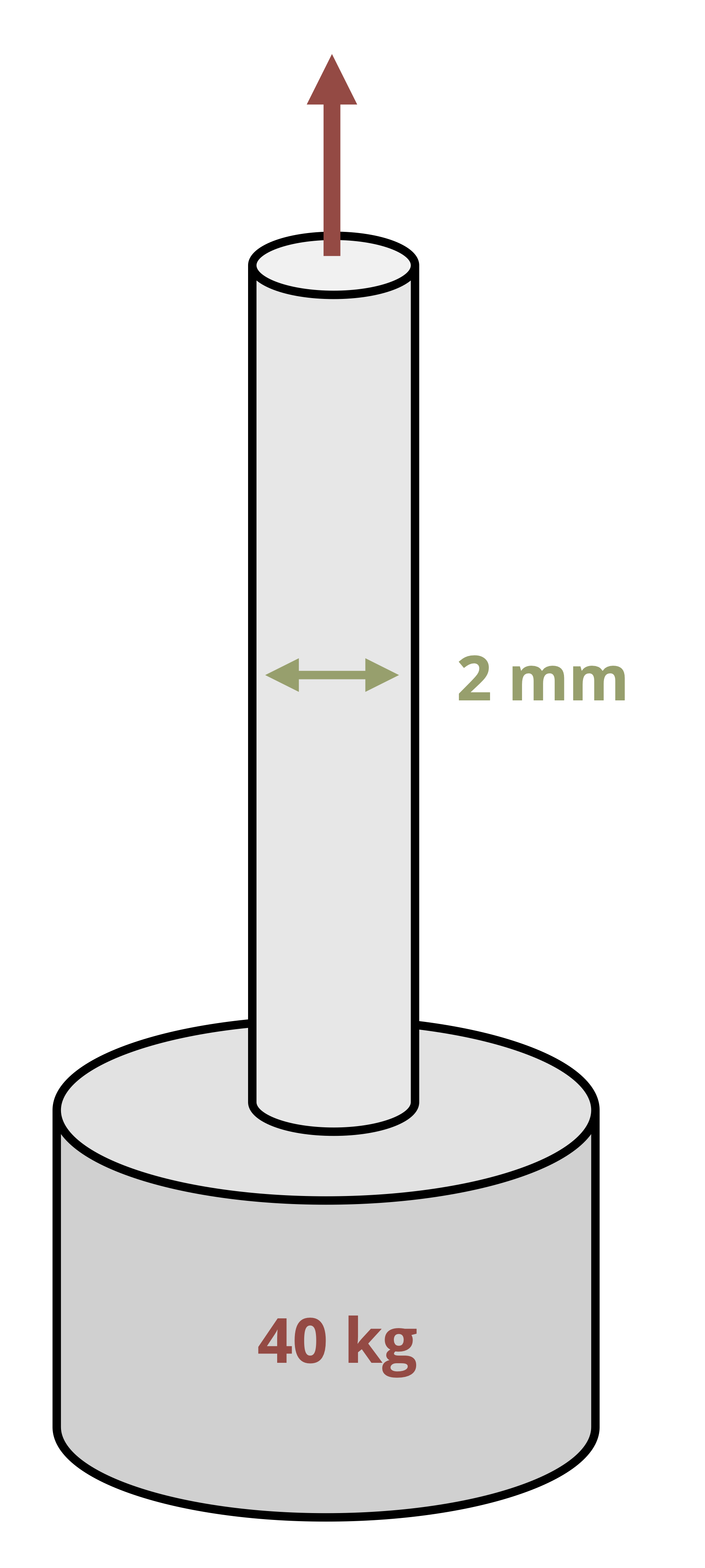
A 2 mm diameter steel wire is used to suspend a mass of 40 kg.

Using the yield strength of 200 MPa as the failure stress, what is the factor of safety of the wire?

TipSolution

First determine the normal force in the wire caused by the mass.

\[ N=40{~kg} * 9.81~\frac{{m}}{{s}^2}=392~\frac{{kg} \cdot {m}}{{s}^2}=392{~N} \\ \]The stress in the wire can be calculated from

\[ \sigma=\frac{N}{A}=\frac{392{~N}}{\pi*(0.001{~m})^2}=124.8{~MPa} \]

Since the failure stress in the wire is 200 MPa, the factor of safety can be determined from

\[ FS=\frac{\sigma_{fail}}{\sigma_{allow}}=\frac{200{~MPa}}{124.8{~MPa}}=1.60 \]

In practice working the other way is also common. Given a material with a known failure stress and a desired factor of safety, we can determine the allowable stress in the component and then design the component to meet this requirement. This is demonstrated in Example 4.7.

TipExample 4.7

Example 4.7  

A square timber column is used to support a deck. The timber has a failure stress in compression of 1,200 psi.

Using a factor of safety of 2.5, determine the required dimensions of the square cross-section if the column experiences a compressive load of 3,000 lb.

TipSolution

Use the failure stress and factor of safety to determine the allowable stress in the column.

\[ \sigma_{allow}=\frac{\sigma_{fail}}{FS}=\frac{1,200~psi}{2.5}=480~psi \]

Next, determine the required cross-sectional area of the column so that the stress does not exceed 480 psi.

\[ \begin{aligned} \sigma&=\frac{N}{A} \\ A&=\frac{N}{\sigma} \\ &=\frac{3,000~lb}{480~psi} \\ &=6.25~in.^2 \end{aligned} \]

Finally, determine the dimension of each side of the square cross-section.

\[ A=L^2 \\ L=\sqrt{A}=\sqrt{6.25} = 2.5~ in. \]

The column cross-section must be at least 2.5 in. on each side so that the stress doesn’t exceed the allowable stress of 480 psi.

We may safely make the dimension larger than 2.5 in., which reduces the stress further but also increases weight and cost. We may not make the dimension any smaller than 2.5 in., as this will result in a stress greater than 480 psi.

WarningStep-by-Step: Factor of Safety

1. Determine the failure stress of the member. Depending on the application, this may be the yield stress or the ultimate stress.
2. Determine the allowable stress in the member from \(\sigma_{allow}=\frac{\sigma_{fail}}{FS}\).
3. Use the allowable stress to calculate the allowable force in the member or the required cross-sectional area, using \(\sigma_{allow}=\frac{F}{A}\).

Summary

Click to expand

NoteKey Takeaways

The mechanical properties of materials need to be known for engineering design purposes. For many applications, the linear elastic properties are the first step in characterizing a material and in determining stresses resulting from imposed displacements or strains and deflections caused by imposed loading scenarios.

Tensile tests of material samples are a common means to measure material behavior, both in the linear elastic region and beyond.

Tensile tests can indicate the normal stress-strain behavior, and the Young’s modulus (or modulus of elasticity) is defined as the slope of the linear portion of this curve.

The proportional limit, elastic limit, and yield point of some engineering materials are quite similar, and yield strength is used throughout the book to denote this region of material response.

Because safe designs often involve using materials below their yield strength, the linear elastic properties—elastic modulus, shear modulus, and Poisson’s ratio—are important parameters for engineering design.

Poisson’s ratio characterizes the coupling between normal stresses in one direction and strains in lateral directions through the generalized Hooke’s law.

The shear modulus (or modulus of rigidity) relates shear stresses and shear strains in the linear elastic region.

The factor of safety is one simple means to quantify how conservative a design may be, an important parameter in engineering design.

NoteKey Equations

Hooke’s law:

\[ \sigma=E \varepsilon_{long} \]

Poisson’s ratio:

\[ \nu=-\frac{\varepsilon_{lat}}{\varepsilon_{long}} \]

Shear stress and strain:

\[ \tau=G \gamma \]

Relationship between E, G, and \(\nu\):

\[ G=\frac{E}{2(1+\nu)} \]

Thermal strain:

\[ \varepsilon=\alpha \Delta T \]

\[ \Delta L=\alpha\Delta TL \]

Generalized Hooke’s law:

\[ \begin{aligned} & \varepsilon_x=\frac{1}{E}\left[\sigma_x-v\left(\sigma_y+\sigma_z\right)\right] \\ & \varepsilon_y=\frac{1}{E}\left[\sigma_y-v\left(\sigma_x+\sigma_z\right)\right] \\ & \varepsilon_z=\frac{1}{E}\left[\sigma_z-v\left(\sigma_x+\sigma_y\right)\right] \end{aligned} \]

\[ {\begin{aligned} & \gamma_{xy}=\frac{\tau_{xy}}{G} \\ & \gamma_{yz}=\frac{\tau_{yz}}{G} \\ & \gamma_{xz}=\frac{\tau_{xz}}{G} \end{aligned}} \] Factor of safety:

\[ FS=\frac{\sigma_{fail}}{\sigma_{allow}} \]

References

Click to expand

Figures

All figures in this chapter were created by Kindred Grey in 2025 and released under a CC BY license, except for

• Figure 4.1: Tensile tests are a common means to measure mechanic properties of materials. A: Credit Instron ®. All rights reserved. Permission granted for this use case. B: David Dillard. 2024. CC BY-NC-SA. C: Mac McCord. 2024. CC BY-NC-SA.
• Figure 4.3: Engineering materials are often loaded beyond yield to permanently deform the material, as in (A) the stamping process for an automotive panel or in (B) the crushing of a weld-bonded hat section used to absorb energy in an automobile accident. A: © Porsche USA. Reproduced under fair use. Retrieved from https://www.autonews.com/suppliers/porsche-deal-lets-tool-supplier-shine. B: © Ford Motor Company. Released under CC BY-NC-SA 4.0.
• Figure 4.4: Results obtained from tensile tests. A: Kindred Grey. 2024. CC BY. B: Sigmund. 2011. CC BY-SA 3.0. https://commons.wikimedia.org/wiki/File:Al_tensile_test.jpg.